veeral does data
Building Mood-Based Spotify Playlists using K-Means Clustering
20 July, 2020Introduction
My music choices and preferences have always been a direct indicator of my current activity, mood, and emotional state. I listen to upbeat hip-hop songs while working out, soft pop music while I'm feeling moody or down, or something in between while working on my data science projects. This project is an attempt to use Machine Learning to identify those moods and build corresponding playlists for each.
If you're interested in my code, you can find it here!
Project Outline
This project has 4 distinct parts:
- Obtain Spotify Data: Use the Spotify API to obtain all my music listening data from the past year.
- Analyze Music Taste: Take a deep dive into my song, artist, and album preferences and how these preferences have fluctuated over the year.
- Predict Different Moods: Analyse audio features such as the acousticness, tempo, and instrumentalness of my song preferences and utilize the K-Means Clustering algorithim to stratify the music into different, defined moods.
- Create Playlists: Develop custom mood-specific Spotify playlists based on my music preferences and mood clusters from the last two parts.
Obtaining Spotify Data
The first step is to obtain the data that will drive the rest of this project. This can be done with the following steps:
- Visit https://www.spotify.com/us/account/privacy/ -- log into Spotify account and scroll to the bottom and request data.
- Receive a downloadable zip file with listening data from Spotify's team in around 1-3 days
- Use python's Spotipy package to access the Spotify API and load data into a Pandas Dataframe
- Acquire Spotify's audio feature data for all my songs:
# Create A Data Frame with Unique Song ID and corresponding song features
my_feature = pd.DataFrame(columns=[
    "song_id","energy","tempo","speechiness",
    "acousticness","instrumentalness","danceability",
    "loudness","valence"
    ])
# For each Song ID in my Spotify-provided listening history,
# import spotify's audio features in DataFrame
for song in songid:
    features = sp.audio_features(tracks = [song])[0]
    if features is not None:
        my_feature = my_feature.append({
            "song_id":song,
            "energy":features['energy'],
            "tempo":features['tempo'],
            "speechiness":features['speechiness'],
            "acousticness":features['acousticness'],
            "instrumentalness":features['instrumentalness'],
            "danceability":features['danceability'],
            "loudness":features['loudness'],
            "valence":features['valence'],
            },ignore_index=True)
The Spotify API audio features are central to my analysis and mood clustering of my music preferences. Attributes like danceability and energy capture differences between faster and slower paced music, while speechiness quantifies each song's focus on words. A high valence indicates positive/happy /euphoric music while low valence quantifies dark/angry/sad music. A complete list of attributes and corresponding definitions can be found here.
My Music Taste Analysis
To best display and understand my data, I utilized the Plotly package for interactive plotting. Let's take a look at some of my music from the past year.
Top Songs
After Hours, by the Weeknd, tops the chart of my most listened to songs of the past year! Even though the song didn't come out till February, I clearly had it on repeat essentially through April. An interesting note about the song is that it is a 6+ minute song, much longer than the average song I listen to (3ish min.) and the measurement variable of "sum minutes listened" rather than "count of times listened" probably worked in its favor.
Top Artists
Post Malone, whom my dad lovingly refers to as, "Post Office Malone", came out as my top artist of the past year. There was a pretty constant stream of various Post songs over my last 12 months. In fact, all three of his albums show up on my top 20 albums list of the past year!
Top Albums
The Weeknd's After Hours album tops the chart of top albums of the past year, which makes a lot of sense thinking back to all the days of cycling through the album on repeat while messing around in my Jupyter Notebooks. Recently, you can see that Polo G's The GOAT has been occupying much of the Jupyter Notebook-ing time.
Using K-Means clustering to predict my different music-listening moods
To create distinct classes to group my musical moods, I use the K-Means unsupervised learning algorthim.
The K-Means clustering algorithim is one of the most popular (and perhaps most intuitive) machine learning algorithims for classifying unlabeled data. It works in the following steps:
- Choose number of centroids
- Initalize the chosen number of centroids at random, or at specified data points.
- Calculate the Euclidian Distance between each point and each centroid, and label each point by it closest centroid.
- For each labeled group, the average point is calculated. This average point becomes the new centroid for the group
- Step (3-4) occurs iteratively until the dataset converges (minimal points switching classes during step 3)
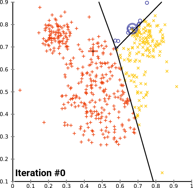
Repeating steps 3-5 until convergence on a 3-cluster, 2D dataset:
Choose the number of clusters
This algorithim works very well, on the basis of choosing a number of centroids that represents the data. There are a few methods to choosing a number of clusters, and in this project I use the elbow method, choosing the number of clusters at the knee of the graph of clusters x inertia (sum of squared distance)
I run the sklearn K-Means algorithim on my data set and ultimately choose 4 clusters based on the graph
Clusters x Inertia
Preprocess the Data
Now that I have an algorithim and process down, I begin the preprocessing of my data! To capture my true preferences, as opposed to songs I listened to for a minute and never again, I filter down my data to songs that I have listened to for more than 15 minutes in the past year.
Dataframe Snapshot
| Song | Artist | Album | Energy | Tempo | Speechiness | Acousticness | Instrumentalness | Danceability | Loudness | Valence |
|---|---|---|---|---|---|---|---|---|---|---|
| No Option | Post Malone | Stoney (Deluxe) | 0.734 | 0.238 | 0.057 | 0.075 | 0.000 | 0.575 | 0.805 | 0.494 |
| My Bad | Khalid | Free Spirit | 0.568 | 0.244 | 0.082 | 0.543 | 0.266 | 0.645 | 0.620 | 0.391 |
| The Show Goes On | Lupe Fiasco | Lasers | 0.889 | 0.606 | 0.115 | 0.018 | 0.000 | 0.591 | 0.855 | 0.650 |
| Escape | Kehlani | SweetSexySavage | 0.688 | 0.213 | 0.079 | 0.039 | 0.000 | 0.562 | 0.787 | 0.707 |
Data Distributions
The first thing I noticed about each feature is that the distributions are all a bit different. Let's visualize this:
A few impressions of the data:
- Instrumentalness is heavily skewed with almost only low values (More lyrical music and electronic beats, less jazz, rock, or heavy metal)
- Speechiness is also skewed toward lower values. More music, less podcasts, speeches, and other spoken word.
- Energy, danceability, and loudness features all have inherently similar, slightly skewed distributions
- Valence and tempo features seems to be the most evenly distributed from 0 to 1.
Run the Algorithim
The data is ready to be fed through algorithim to develop the mood clusters!
# Drop non-numeric columns
# Convert Dataframe to a numerical Numpy array
X = df.drop(['track_name','artist_name','album'],axis=1).values

# Fit data to 4 clusters using the sklearn K-Means algorithim
from sklearn.cluster import KMeans
kmeans = KMeans(n_clusters=4,n_jobs=-1).fit(X)

# Predict and label mood for each song in Dataframe
kmeans_mood_labels = kmeans.predict(X)
df['label'] = kmeans_mood_labels
Visualize the Results
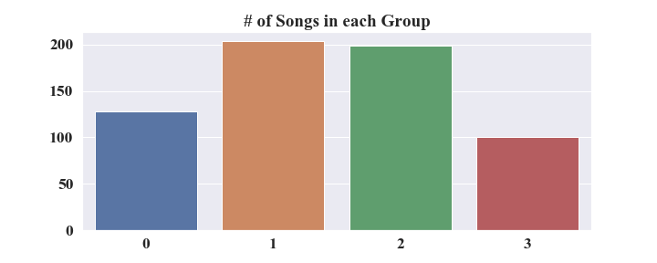
My algorithim produced the following cluster value counts:
PCA - 2D
Each song in my dataframe has 8 audio features, which essentially means the data is 8-dimensional. Because data cannot by visualized in 8 dimensions, I used a common dimensionality reduction technique called Principal Component Analysis (PCA) to condense my data into 2 dimensions in a way that maintains as much of the original data's variance as possible.
Using sklearn's PCA package:
from sklearn.decomposition import PCA
pca_2d = PCA(n_components=2)
principal_components = pca_2d.fit_transform(X)
pc_2d = pd.DataFrame(principal_components)
pc_2d.columns = ['x', 'y','label']
(It is important to note that (x,y) coordinates plotted are a transformed representation of a combination of my 8 features, but do not exhibit any direct intuition into the feature values)
By using PCA, I can see my data much more clearly. As shown in the plot, labels "2" and "3" are pretty well defined with not too much overlap, while labels "0" and "1" have a large amount of overlap.
Input: print (pca_2d.explained_variance_ratio_ , sum(pca_2d.explained_variance_ratio_))Output: array([0.32387322, 0.22293707]), 0.5468Using the above PCA attribute, I see that 32% of my data's original variance was explained by the 1st component while 22% is explained by the 2nd. Altogether, my PCA reduced the dimensionality the 8 features while maintaining around 54% of the original variance.
PCA - 3D
Next, I reran my PCA function, this time with three components, using Plotly's 3D Scatter Plot functionality to display my data. The cluster stratifications are much clearer now, with the 3rd component capturing an extra 17.5% of the original data's variance. This 3-component transformation of the 8 feature data exhibits a much clear visual cluster distinction while maintaining more than 77% of the original variance.
pca_3d = PCA(n_components=3)
principal_components = pca_3d.fit_transform(X)
pc_3d = pd.DataFrame(principal_components)
pc_3d.columns = ['x', 'y', 'z', 'label']Input: print (pca_3d.explained_variance_ratio_ , sum(pca_3d.explained_variance_ratio_))Output: array([0.32387322, 0.22293707, 0.17594222]), 0.7226Results
Now that I've analysed my mood clusters, I am going to try and define each mood! To do this, I will do the following:
- Summarize the cluster's audio feature statistics
- Try to define a respresentative mood
- Look at a sample of the song data for manual confirmation
First, I scale all of my data features using the sklearn Standard Scaler. The scaler will transform each audio feature value such that each audio feature has a mean of 0 and variance of 1 across all songs in the feature column. This will allow for a much clearer visualization of comparing features for each cluster.
I now visualize the feature differences using seaborn's heatmap plot:

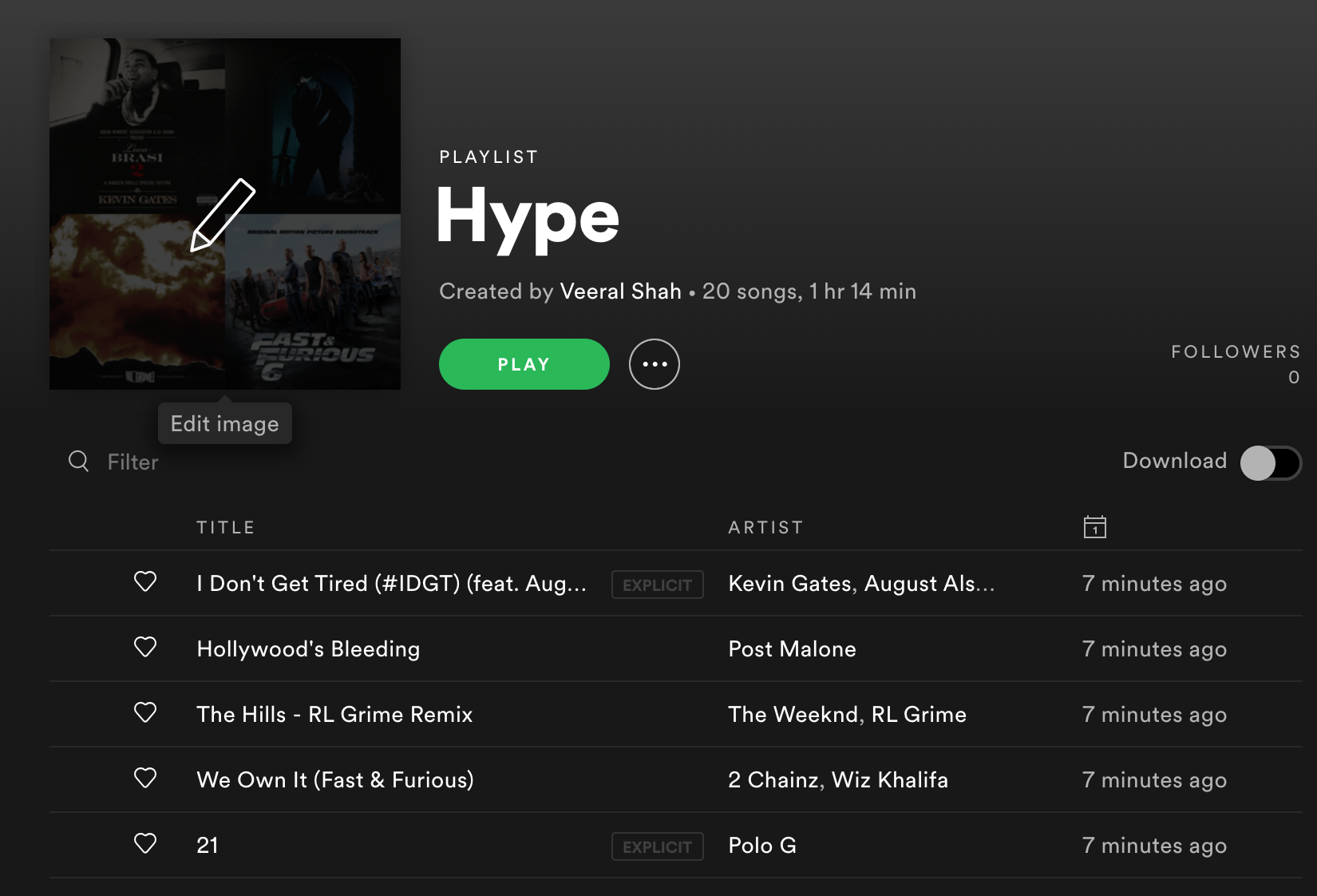
Cluster 0: HYPE mood

Cluster 0 seems to be exciting, fast paced songs with a lot of words. Its audio features are:
- Very High Speechiness and Tempo
- High Loudness and Energy
- Semi-Low Danceability
These audio features point to the mood cluster contain a lot of Lyrical, Hype Rap songs. A quick random sample immediately confirms that:
| Song | Artist | Album | Label |
|---|---|---|---|
| iPHONE (with Nicki Minaj) | DaBaby | KIRK | 0 |
| XO Tour Llif3 | Lil Uzi Vert | Luv Is Rage 2 | 0 |
| I'm Goin In | Drake | So Far Gone |
0 |
| Flex (feat. Juice WRLD) | Polo G | THE GOAT | 0 |
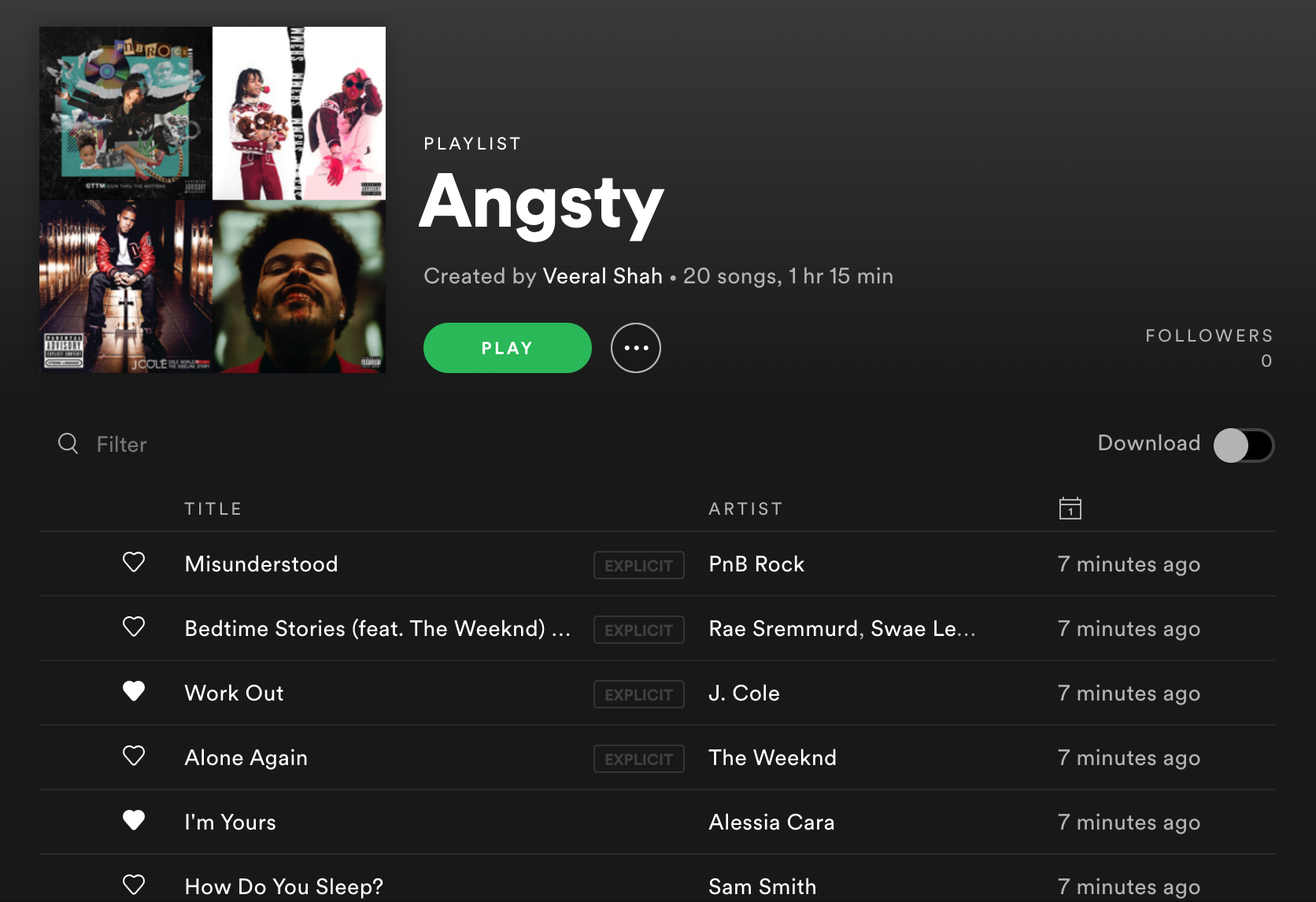
Cluster 1: ANGSTY mood

Cluster 1 is perhaps the most ambiguous mood cluster. Its audio features are:
- Very Low Tempo and Valence
- Low Instrumentalness and Acousticness
- Average Energy and Danceability
These songs are not particularly positive, but are not instrumental/acoustic sad songs either. The average energy and danceability makes me feel like the cluster's songs are catchy but a little more angsty and not quite as hype as Cluster 0.
These audio features point to the mood cluster containing a lot of Moody Pop/R&B Songs. Here's a random sample of songs in the cluster:
| Song | Artist | Album | Label |
|---|---|---|---|
| One Dance | Drake | Views | 1 |
| Too Late | The Weeknd | After Hours | 1 |
| Own It (feat. Ed Sheeran) | Stormzy | Heavy Is The Head |
1 |
| EARFQUAKE | Tyler, The Creator | IGOR | 1 |
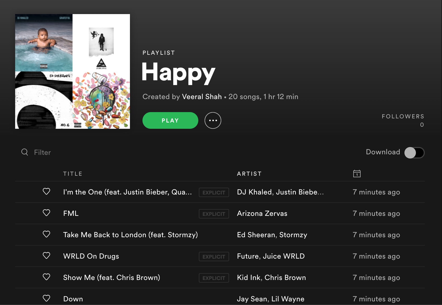
Cluster 2: HAPPY mood

Cluster 2 was similar to Cluster 0 in loudness and energy, though specifically different in speechiness and danceability. Its audio features are:
- Very High Danceability and Valence
- High Loudness and Energy
- Low Instrumentalness
These songs are happy and exciting and make you want to dance. However, unlike Cluster 0, the songs do not have a high speechiness.
These audio features point to the mood cluster contain a lot of Upbeat Happy Pop - catchy songs you can sing and dance to. Here's a random sample of songs in the cluster:
| Song | Artist | Album | Label |
|---|---|---|---|
| Medicated (feat. Chevy Woods & Juicy J) | Wiz Khalifa | O.N.I.F.C. (Deluxe) | 2 |
| Break My Heart | Dua Lipa | Future Nostalgia | 2 |
| Loyal (feat. Lil Wayne & Tyga) | Chris Brown | X (Expanded Edition) |
2 |
| Juice | Lizzo | Cuz I Love You | 2 |
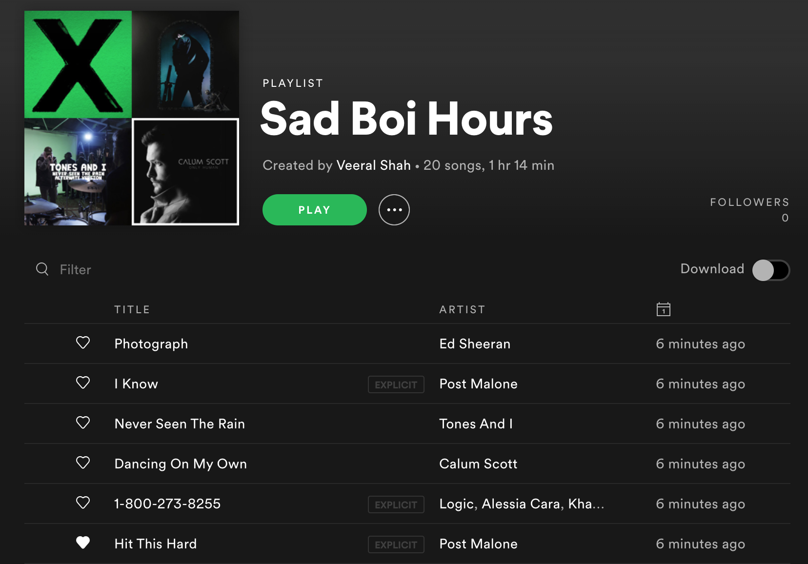
Cluster 3: GLOOMY/EMOTIONAL mood

Cluster 3 was probably the easiest mood for me to identify. Here are the audio features:
- Very High Acousticness and Instrumentalness
- Very Low Loudness and Energy
- Low Danceability and Speechiness
These songs are slow and emotional. The audio features point to the mood cluster containing songs in a mood I would probably call my Sad Boi Hours. Here's some sample songs:
| Song | Artist | Album | Label |
|---|---|---|---|
| Vertigo | Khalid | Suncity | 3 |
| Hold Me By The Heart | Kehlani | SweetSexySavage (Deluxe) | 3 |
| Summer Friends (feat. Jeremih & Francis & The Lights) | Chance the Rapper | Coloring Book |
3 |
| FourFiveSeconds | Rihanna | FourFiveSeconds | 3 |
Creating Mood-Based Playlists in Spotify
Using Spotipy's playlist access with the scope "playlist-modify-public", it is possible to create Spotify playlists right from a Jupyter Notebook!
from spotipy.oauth2 import SpotifyOAuth

scope = 'playlist-modify-public'
token = util.prompt_for_user_token(username=username,
                                   scope=scope,
                                   client_id=client_id,
                                   client_secret=client_secret,
                                   redirect_uri=redirect_uri)

sp = spotipy.Spotify(auth_manager=SpotifyOAuth(client_id,client_secret,redirect_uri,scope=scope,username=username))
def create_mood_playlists(moods, df, num_clusters, playlist_length):
'''
Input: List of defined moods, features df, number of clusters, len of desired playlist
Output: Spotify Playlist
'''
for moodnum in range(num_clusters):
mood_data = df[df.label==moodnum]
sp.user_playlist_create(username, moods[moodnum])
playlist_id = sp.user_playlists(username)['items'][0]['id']
playlist_song_IDs = list(mood_data['track_id'].sample(playlist_length))
sp.user_playlist_add_tracks(username, playlist_id, list(playlist_song_IDs))
moods = ['Hype','Angsty','Happy','Sad']
num_clusters = 4
playlist_length = 20
create_mood_playlists(moods, song_prefs, num_clusters, playlist_length)Check 'em out!
Next Steps
Build a Web App that, when given Spotify username and token access info, the app will run the K-Means Algorithim, create defined moods, and then build custom mood-specific playlists for the user directly in the Spotify app.